Regime maps
In (Llimona, 2015) we introduced a concept, back then called Playability Map, that deserves more elaboration. Its meaning is clearer as a regime map, as we will see shortly.
A regime map is a (usually two-dimensional) visual representation of how certain aspects of the model and gesture spaces map to the acoustic space. In a regime map, two dimensions from one of the mentioned spaces form a matrix, based on which and a heat map indicates the value of a particular acoustic space dimension – usually a value within a particular regime set. The Schelleng diagram is actually one of the possible regime maps one could build, which sweeps the bow force and bow-bridge distance dimensions of the gesture space across a pre-defined, log-spaced range, and looks at how the sound changes by employing a few symbolic descriptors: good, surface, and raucous sound.
Given a digital simulation of a bowed string and a regime estimator, it is straightforward to compute a numerical regime map by running the estimator on notes played under all the desired conditions. Not only that, but synthesizing a sound given some parameters and estimating the regime of vibration is something that can be done completely independently for all needed parameter combinations, which provides an embarrassingly parallel setup.
This concept of building a “Schelleng diagram” by analyzing vibration regimes is mentioned in (Woodhouse, 2004), where the authors use this method for testing models with alternative friction formulations. Other authors use completely different regime maps, with (Guettler, 2002) being a notable example with his representation of the time before Helmholtz triggering, which is the regime descriptor, depending on the bow force and acceleration. (Schoonderwaldt, 2008) even build an empirical regime map by bowing an actual instrument using a machine.
Regime map descriptors
Once we have a regime map, it is possible to define metrics that describe the map itself, that is, that quantify the mapping between the model or gesture space and the acoustic space. This is highly relevant, because effectively quantifies what players pay attention to when playing: how what they do is translated into sound.
These descriptors depend a lot on the particular regime map we are looking at. In the Schelleng space, several interesting features can be extracted, such as the slope of the minimum and maximum bow forces, which are supposed to be close to the well-known theoretical result.
These descriptors could range from just extracting a function over a one-dimensional domain from the two-dimensional domain of the map to obtaining a single number that describes it, and then computing several maps changing third variables in order to see how this descriptor changes. We would then have a spatial mapping map, that shows how the relationship between some aspects of the model or gesture spaces and the acoustic space change when another aspect of the former is modified. This could be regarded as a higher-level regime map.
It is using these higher-order representations that the concept of playability can arise again and be approached from a quantitative perspective, since in some cases the descriptors will precisely tell how nice the mapping between gestures and sound is, and then we will be able to study their dependence on the model. An example of a descriptor that probably correlates with how playable a model is would be the Helmholtz Region Dynamic Range, which consists on the difference in dB between the minimum and maximum bow forces for a given bow-bridge distance in the Schelleng map.
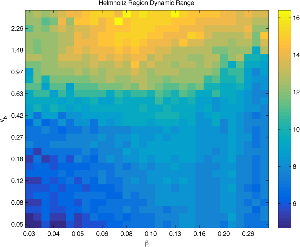 Higher-order mapping map constructed by computing a one-dimensional descriptor of the Schelleng map, the Helmholtz Region Dynamic Range, multiple times using different bow velocities.
The minimum force map descriptor
In this project, we will be using a helmholtzness regime set in order to know whether we have Helmholtz motion or not, and for each desired configuration of study (different pitches that will change where the spectral content of the sound falls on the admittance) we will simulate performance with many different bow force values. As a descriptor, we will keep the lowest force that achieves Helmholtz motion for each of the simulated pitches.
In reality, it is not the lowest force that achieves Helmholtz motion that we keep, but the highest force that does not achieve it before entering the raucous region. We chose to do this because many times there are regions that display Helmholtz motion between a region with continuous slipping due to the bow not even sticking to the string and another region with multiple stick-slip cycles. According to the literature, the transition into the Helmholtz region happens after multiple stick-slip cycles are no longer feasible.
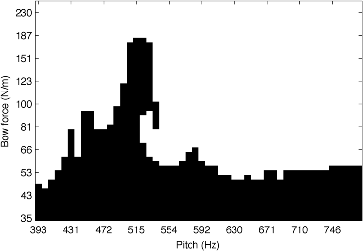 Regime map that shows where the vibration is on the helmholtzness regime set, depending on the bow force and the expected pitch.
Issues when using pitch as a map dimension
When one of the desired dimensions of the regime map is pitch, it is important to make a distinction between expected and resulting pitch. In many cases, the resulting pitch does not correspond to the one would expect given the string length, tension and modulus, because of flattening effects. The situation gets even worse if there is numerical detuning, as it is common in low-resolution delay line interpolation.
In our case, there was not too much flattening because the bow force was very low, but we had severe numerical detuning in some cases. What we did was to, for each expected pitch, select one of the simulations with different bow force half-way between the detected minimum bow force and the maximum we had, detect its pitch using the YIN algorithm, and use that pitch in all further analysis steps.