Results
In order to test whether the prediction by Woodhouse and our simulations are in agreement with respect to the minimum required bow force, we swept a synthesizer implementing the model described in (Maestre, 2014) playing different pitches over a range of an octave on the D string using the same parameters that Woodhouse had used in the analytical study.
By using driving-point admittance data measured experimentally in previous studies and fitted into the model to match its bridge structure (Maestre, 2013), the synthesizer effectively played using 10 different violins – and for each of them we computed the expected minimum force according to the analytical formulation.
The following plot shows that the analytically expected and simulated data are in high agreement.
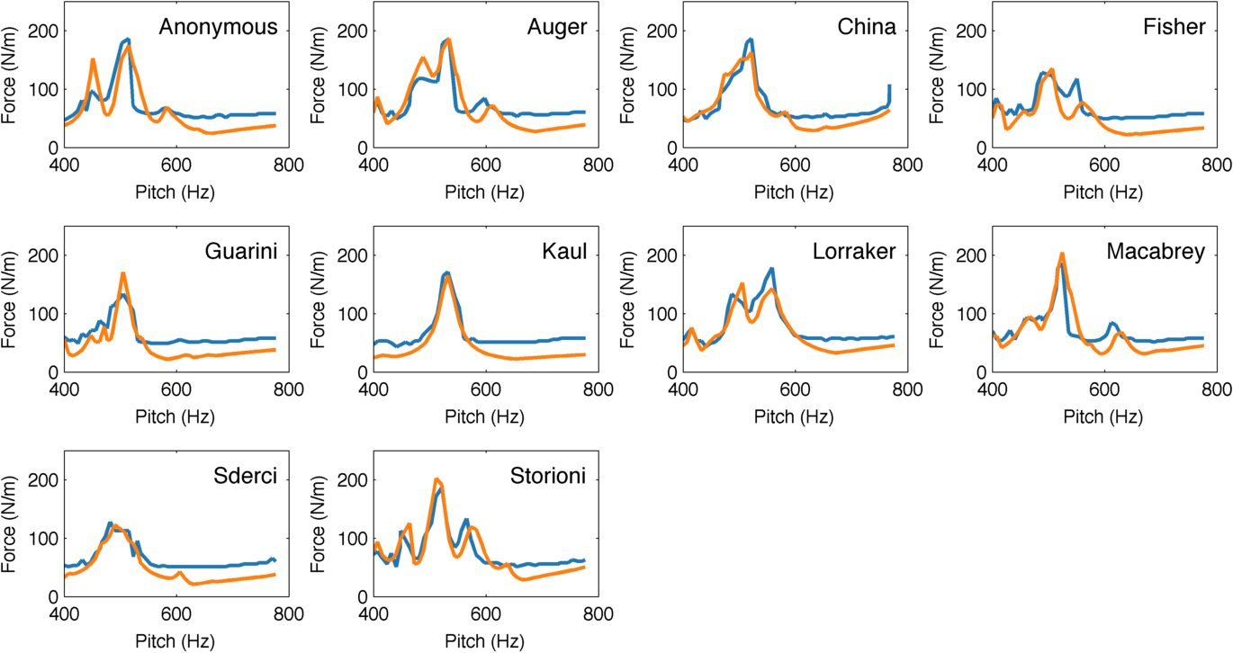 Simulated (blue) and theoretical (orange) minimum bow forces when playing notes with a different pitch on different instruments. Each one of the subplots represents an instrument, characterized by its driving-point admittance.
Indeed, the Pearson correlation coefficient between expected and simulated minimum forces is quite strong for all of the instruments. However, this is a very localized study that only look at a range that spans 200 Hz. We plan to expand the analysis to other pitch ranges, although it will have to use a different string for playing to keep a usable string length.
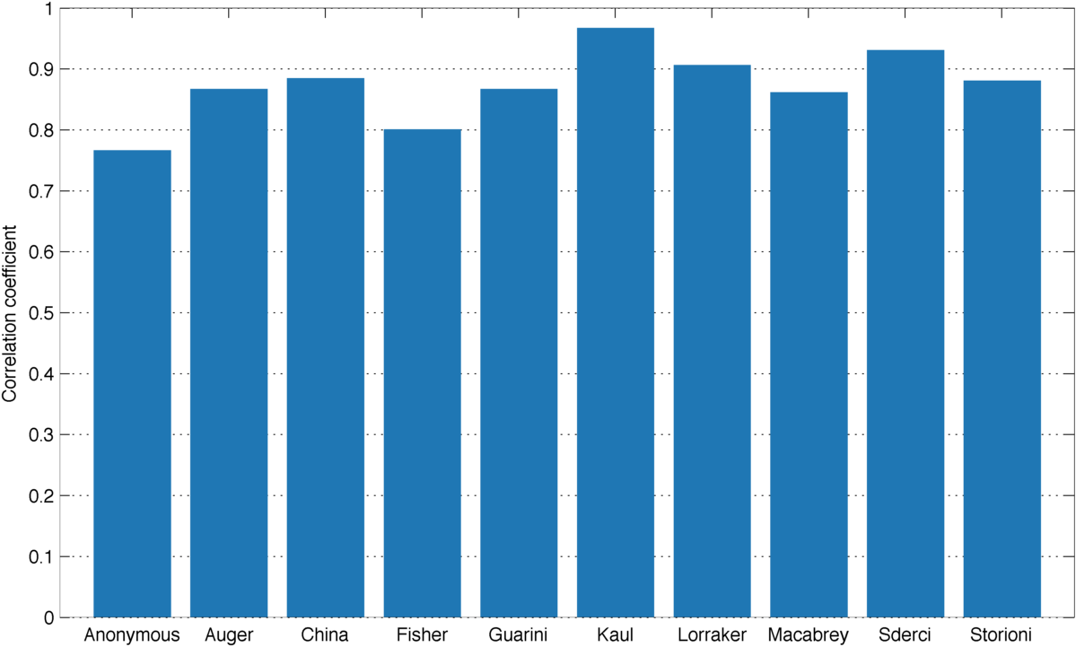 Correlation between simulated and theoretical minimum bow forces.
It is also interesting to look at the cross-correlation matrix that shows how correlated is the theoretical minimum force of each violin to the measured one on all the violins. If the models agree, we should expect the correlation for the same violin to be higher than across two different violins, which is mostly the case.
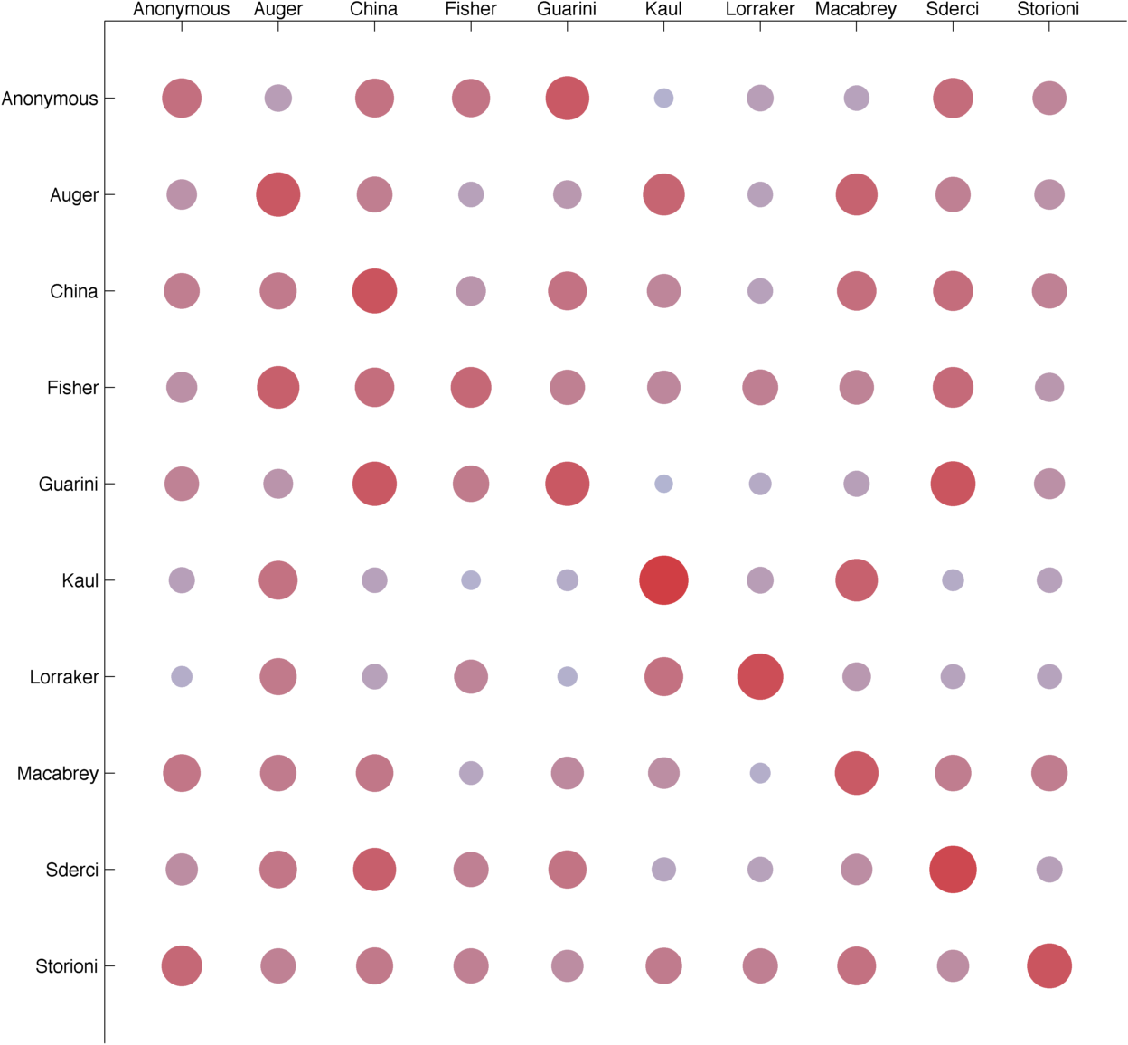 Matrix that shows how correlated the theoretical minimum force of a violin is to the measured one on all the others, including itself on the diagonal.
However, correlations using different violins are quite high for a very simple reason: all violins have similar shapes and materials, and those are what determine the resonance modes, which provide the frequency-dependent component of the admittance. In other words, the admittances themselves correlated across different violins.
Critique
One of the most interesting features of this project is that it compares directly predictions made by two models that make completely different assumptions about how friction works in bowed strings. The Raman model used when deriving the theoretical results assumes dry friction, with a (constant) static friction coefficient that applies during stick and a (constant) dynamic friction coefficient that applies during slip. However, the numerical synthesizer uses a viscous formulation of friction, assuming that rosin is a highly viscous liquid. Since the melting point is very close to ambient temperature, the friction coefficient varies a lot during performance due to the heat generated by friction itself.
What this means in practice is that the formula cannot be applied as-is. In the simulations, the friction coefficient can vary between 0.4 and 1.2, depending on temperature. However, using this range yields completely unrealistic results because such a variation only happens when the bow force is very high, and therefore the contact heats up a lot. In the range of bow forces we have studied, the friction coefficient never drops below 1.0.
In the results we used a difference between equivalent static and dynamic friction coefficients of 0.05, which seems to give a good match between the predicted and measured minimum bow forces. From this, we tried to find an explanation for that value.
In a dry friction model, the difference between static and dynamic friction is what defines the two different stages of the oscillation; during stick, static friction applies, and when the restoring force of the string imposed by the incoming wave overcomes friction, the string starts slipping and dynamic friction applies.
When studying the bow force limits, the only relevant thing is whether this phase transitions from stick to slip occur as we would like them to. Therefore, we should pay attention to what happens at the exact moments when the string is captured and released. If we look at the value of the friction coefficient in the viscous friction model in those moments, we observe that it is very consistent and localized.
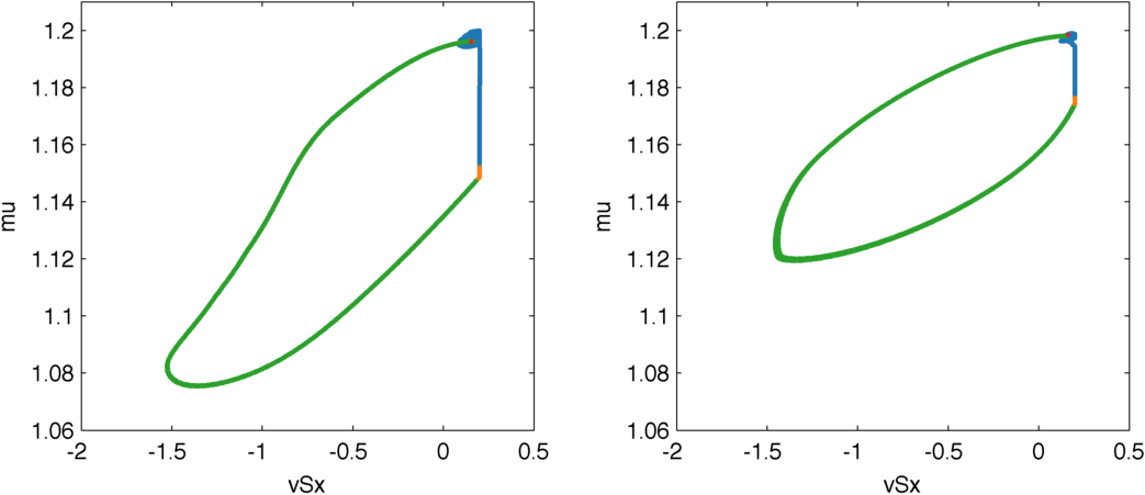 Evolution of the friction coefficient depending on the differential string velocity, displaying a hysteresis curve. During stick, there is no differential velocity and the friction increases due to cooling (blue). When the string is released (red), slip begins. During slip (green), the differential velocity heats up the contact and the friction lowers. But this lowering produces a smaller friction force, so the contact stops heating and the friction increases again, until the string is captured (orange).
Therefore, it makes sense to use those values as the equivalent static and dynamic friction coefficients. The problem is that they depend on the bow force, therefore we will get different equivalent dry friction coefficients depending on what we assume is the minimum bow force (which is in turn what we are trying to estimate).
Our approach here was to take the coefficients using the bow force that the simulation said was the minimum. This is introducing data about our predictions into the analytical expression, so the results would not be very reliable, but it should show if working with equivalent friction makes sense.
In the plot we see that at high pitch the equivalent friction coefficient difference is very small, and that could explain why we were overestimating the minimum bow force there – this difference is at the denominator in the formula. However, just plugging this data into the formula does not work; the results are far off by several orders of magnitude.
That being said, the value that we had guessed of the coefficient difference being 0.05 appears to make sense with what the plot shows, since while the maximum is near 0.2 the mean is much closer to what the used.
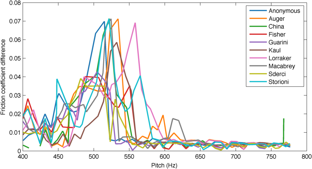 Equivalent friction coefficient difference for each violin and pitch computed by probing the friction coefficient at relevant locations.